As explained in the pages on digital cameras, most sensors record color images in terms of their red, green and blue intensities. So do human eyes, whose three types of color receptors (cones) respond to somewhat overlapping ranges of wavelengths that are commonly characterized as red, green and blue. Images are stored in the computer in terms of their red, green and blue (RGB) intensities, and displayed on CRT monitors with RGB phosphors or on LCD flat screens with RGB filters.

But human perception of colors does not describe them in terms of their RGB components, and the stored RGB channels rarely provide optimal contrast or an appropriate color space for image processing. Other sets of color coordinates are available that provide better results. Two of the most widely used are hue-saturation-intensity (HSI) and LAB. There are several variants of each, but the diagrams in Figure 1 identify the basic geometries.

HSI coordinates provide a central axis (I) that ignores color altogether and measures the brightness (sometimes described as intensity or luminance) of the pixels in the image. For a monochrome or gray scale image, with no color, all of the pixel values would plot along that central axis. When color is present, pixel values move off the axis. The distance that they are displaced is a measure of the amount of color, or saturation (S). A maximum saturation color such as pure red may be compared to a less saturated color such as pink. Hue (H) is represented in this space as an angle, which progresses around the color wheel from red to yellow, then green, cyan, blue, magenta and back to red. This is the familiar color wheel children learn about and artists use.

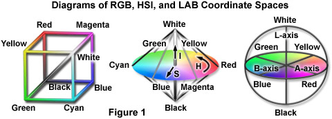
Notice that the HSI coordinates shown in the diagram have a bi-conical shape that tapers to a point at white and another one at black. A maximum brightness value is produced on your computer display by setting red, green and blue brightnesses to maximum. The only way to introduce color (i.e., increase saturation) is to reduce one or more of the individual colors. Similarly, at the black point the RGB values are zero, and saturation can only be increased by increasing brightness. The variation of maximum saturation with brightness is one of the mathematical problems with HSI spaces.

Another problem is the wrap-around of the hue angles. A color slightly to the orange of red (e.g. 10°) and one slightly to the magenta of red (e.g. 350°) should average out to red (0°), but arithmetically the average is 180° (cyan). So special modulo arithmetic is involved.

Although computer programs can handle these complications, another somewhat simpler space is also widely used. The spherical LAB space shown in the diagram has orthogonal axes that make arithmetic easy. The L (luminance) axis is the vertical line from the south to the north pole, and just as the (I) axis in HSI space, L corresponds to brightness with no color. The A and B axes are (red - to - green) and (yellow - to - blue) respectively. The equatorial plane in this space is also a color wheel, although it is somewhat twisted as compared to that in the HSI coordinates.

	Interactive Tutorial
Color Sampler Click on any point in an image to read out the RGB, HSI and LAB values.

The Color Sampler interactive tutorial compares these color coordinates. The HSI or LAB channels (see the Color Channels interactive tutorial) often provide better ways to examine and interpret the contents of images than do RGB. For example, hue corresponds to the color of various stains and fluorescent dyes or proteins, while saturation corresponds to the amount of the stain or dye present and intensity in a transmission image of a thin section is a measure of local density. LAB channels correspond approximately to the ways that color television signals are broadcast and adjusted.

	Interactive Tutorial
Color Channels Examine any color channel in RGB, HSI, and LAB color spaces to see how the image contrast varies.

For processing of color images, converting the image from RGB coordinates to either HSI or LAB, processing only the brightness values, recombining the modified brightness with the original color, and converting back to RGB so the result can be displayed is almost always the preferred method. Processing the individual RGB channels alters the proportions of those colors and produces color shifts and distortions that are visually distracting. The Laplacian Sharpening interactive tutorial compares the results of sharpening the L channel to sharpening the individual RGB channels. Most of the examples that follow in this tutorial process the intensity or luminance information and preserve the colors.

	Interactive Tutorial
Laplacian Sharpening Compare sharpening of an image by using RGB channels versus the LAB L channel.

The use of alternative color coordinates offers opportunities for filtering to achieve improved contrast, both to visually reveal structures that are present and potentially to make them easier to discriminate for subsequent measurement. For example, it is possible to apply an arbitrary color filter to an image after it has been acquired. The brightness of a filtered image is the dot-product of the color vector of each pixel (RGB components) with the color vector of the filter (defined by its hue). The Hue-Based Grayscale Conversion interactive tutorial demonstrates the effect of different filter colors (hues) on images.

	Interactive Tutorial
Hue-Based Grayscale Conversion Apply colored filters to generate a grayscale image and manipulate image contrast.

Many programs also allow arbitrary mixing of channels to improve contrast. A combination of about 65 percent green, 25 percent red, 10 percent blue produces a monochromatic image whose brightness corresponds to the human visual impression of brightness, rather than a simple averaging of the red, green and blue. However, in many cases arbitrary combinations, including negative amounts of one or two channels, may be useful to highlight specific structures. In the RGB Channel Mixer interactive tutorial, an optional autoscaling feature automatically adjusts the values to total 100 percent.

	Interactive Tutorial
RGB Channel Mixer Combine arbitrary proportions of red, green, and blue to generate a grayscale image.

For any image there is a unique optimal combination of channel mixing weights that produces the greatest amount of contrast. The line that corresponds to this axis (called the principal components axis) in color space is the one that best fits the cloud of data points representing the color coordinates of all of the image pixels. This can be determined by regression. As shown in the PCA Grayscale Conversion interactive tutorial, the principal axis produces excellent monochrome contrast in some images (but not all).

	Interactive Tutorial
PCA Grayscale Conversion Explore grayscale conversion of a color image using principal components analysis.

---

BACK TO INTRODUCTION TO DIGITAL IMAGE PROCESSING AND ANALYSIS

BACK TO MICROSCOPY PRIMER HOME

Questions or comments? Send us an email.

© 1998-2009 by Michael W. Davidson, John Russ, Olympus America Inc., and The Florida State University. All Rights Reserved. No images, graphics, scripts, or applets may be reproduced or used in any manner without permission from the copyright holders. Use of this website means you agree to all of the Legal Terms and Conditions set forth by the owners.

This website is maintained by our
Graphics & Web Programming Team
in collaboration with Optical Microscopy at the
National High Magnetic Field Laboratory.

Last modification: Tuesday, Sep 11, 2018 at 01:16 PM

Access Count Since July 20, 2006: 15886

For more information on microscope manufacturers,
use the buttons below to navigate to their websites: