There are four basic classes of measurements on individual features: those involving the pixel values (color, brightness, or derived values such as density); measures of size (such as area, diameter, perimeter or length); information on position (either absolute coordinates, or position relative to other objects); and finally values that characterize shape.

Digital cameras record color information as red, green and blue components. Each filter passes a broad range of wavelengths, so there is no way to determine what the actual colors of light emitted, transmitted or reflected from the sample may be. However, since human vision also uses three detectors, each of which also responds to broad (and overlapping) wavelength ranges, it is generally possible to perform color matching so that the visual impression of color from the recorded image (as displayed or printed) is the same as that of the original scene. This is, of course, vital to publishers of catalogs, whose customers expect to get what they see.

In most microscopy and other scientific applications, it is not necessary to actually measure the color (if it is, it is necessary to use a spectrophotometer, not a digital camera). The hue-saturation-intensity values of colors may, however, be useful for purposes of feature selection. In the Color-Based Feature Counting interactive tutorial, candies were imaged by placing them on a flatbed scanner. Counting based on color required both the hue and intensity values in order to distinguish orange from brown, as shown in the table. Click on each line in the table to see the selected objects.

	Interactive Tutorial
Color-Based Feature Counting Identify and count objects based on HSI color values.

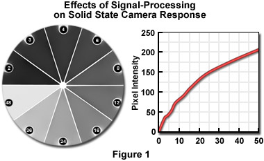
Density can be measured using a digitized image provided that appropriate calibration is performed. Unfortunately, that must usually be done frequently because of aging of light sources and electronic components, the effects of minor changes in line voltage, and any variations in optical setup. Although the solid-state sensors used in digital cameras are inherently linear, the amplifying electronics, digitization, and any post-processing can alter the response as shown in Figure 1.

There are several candidate parameters to describe feature size. The area, determined by counting pixels and often expressed as the “equivalent diameter” (the diameter of a circle with the same area), is widely used. But for some applications other diameters, such as that of the largest inscribed or smallest circumscribed circle, may be more appropriate. Length is usually determined as the greatest distance between any two points in the object, but for a long, curved object like a fiber the length of the skeleton is more meaningful, and there are a great many alternative definitions for breadth. The perimeter of objects is difficult to determine because (except for some smooth objects such as those bound by a membrane or surface tension) the resolved perimeter usually increases in length with magnification.

Whatever measure of size is chosen, determining the values is typically performed on a binary (black and white) image after any necessary processing such as filling of holes, morphological smoothing, rejection of small features due to dirt or noise, watershed separation, and so on. The Describing Feature Size interactive tutorial illustrates several typical sequences by which data are obtained and presented. Calibration may be performed by imaging a stage micrometer. Statistical analysis is often performed on the resulting data.

	Interactive Tutorial
Describing Feature Size Measure and report size distributions of image features.

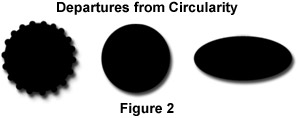
Size is generally a well-understood property, even if there can be several measurement definitions. Shape is more difficult because there are few common words to describe shape, and even fewer agreed-upon measurements. Two of the most widely used parameters are roundness and formfactor, defined by the relationships in Equation 1 (but note that not all systems use either of these exact definitions - numeric constants may be omitted or the reciprocal values used - and sometimes the names are interchanged!).

(1)

These two parameters both calculate 1.0 for a perfect circle and measure two different ways that a shape can vary from circularity. But as shown in Figure 2, one (Roundness) responds to elongation while the other (Formfactor) detects irregularities. And, of course, there can be many other ways to “not be a circle.”

In the Feature Shape Descriptors interactive tutorial, measurement of roundness is used to characterize the shape of starch granules, while a correlation between formfactor and size for the powder sample indicates that the larger particles are actually agglomerates of smaller ones and that this accounts for their more irregular shapes. There is an almost unlimited number of combinations of size measurements for which the dimensions formally cancel, and any of these may be useful in a particular situation, if one can be found.

	Interactive Tutorial
Feature Shape Descriptors Measure feature shapes and report results.

Two characteristics of shape that are often recognized by humans are topology and boundary fractal dimension. The first of these is captured by the feature’s skeleton. As shown in the Topological Shape interactive tutorial, the number of points in each star-shaped feature is instantly recognized by the viewer, and corresponds to the number of end points in the skeleton. That property can be used as shown to label the features.

	Interactive Tutorial
Topological Shape Use the skeleton to characterize feature shape.

Fractal dimension is a measure of the self-similar irregularity of the feature boundary, without regard to its topological shape. Smooth objects with boundaries controlled by membranes or surface tension have a dimension of 1.000, but as the boundary becomes more irregular and the feature tends to spread over the plane, the value rises as shown in the Fractal Shape interactive tutorial. Many correlations between this dimension and pathology of cells, history of particle erosion, chemical kinetics, and other processes have been reported.

	Interactive Tutorial
Fractal Shape Measure the fractal dimension to characterize boundary roughness.

Location is usually based on the centroid (or sometimes the density-weighted centroid) of each feature. In a few instances, the absolute coordinates of features on the microscope slide are important (for example in tracking object motion). Usually, however, it is the tendency for objects to be clustered or self-avoiding that is most interesting. By comparing the mean nearest neighbor distance for the features to that which would be expected if they were independently and randomly dispersed in the image, the spatial distribution of features can be quantified.

(2)

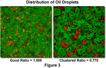
For a random dispersion of N features in an area A, the mean nearest neighbor distance is given by Equation 2. Clustering (e.g., students at a party, cities on a map, particles attracted chemically or electromagnetically) produces a lower measured mean nearest neighbor distance. Conversely, self-avoidance (e.g., students in class, cacti in the desert, precipitate particles that deplete the surrounding matrix) produces a larger measured value. Figure 3 compares the distribution of oil droplets in custard when the mixing is good (near-random distribution) vs. not (the clustering produces an oily texture). The ratio of the measured value to that predicted for the random case is shown.

By measuring a variety of color, size, shape and position values for populations of objects, it is possible to use regression or neural net techniques to train image processing systems to perform automatic feature recognition. This has been used in applications ranging from defect recognition in manufacturing to diagnosis in medicine.

---

BACK TO INTRODUCTION TO DIGITAL IMAGE PROCESSING AND ANALYSIS

BACK TO MICROSCOPY PRIMER HOME

Questions or comments? Send us an email.

© 1998-2009 by Michael W. Davidson, John Russ, Olympus America Inc., and The Florida State University. All Rights Reserved. No images, graphics, scripts, or applets may be reproduced or used in any manner without permission from the copyright holders. Use of this website means you agree to all of the Legal Terms and Conditions set forth by the owners.

This website is maintained by our
Graphics & Web Programming Team
in collaboration with Optical Microscopy at the
National High Magnetic Field Laboratory.

Last modification: Tuesday, Sep 11, 2018 at 02:52 PM

Access Count Since July 20, 2006: 8961

For more information on microscope manufacturers,
use the buttons below to navigate to their websites: