Application of a suitable background subtraction algorithm is a useful technique for correcting image defects that are associated with nonuniform brightness, often (but not always) attributed to uneven illumination in the microscope. This interactive tutorial explores a background subtraction image processing technique that relies on the creation of a background image from the original digital image.

	Interactive Java Tutorial
ATTENTION Our servers have detected that your web browser does not have the Java Virtual Machine installed or it is not functioning properly. Please install this software in order to view our interactive Java tutorials. You may download the necessary software by clicking on the "Get It Now" button below.

The tutorial initializes with a randomly selected specimen image, captured in the MIC-D digital microscope, appearing in the left-hand window entitled Specimen Image. Each specimen name includes, in parentheses, an abbreviation designating the contrast mechanism employed in obtaining the image. The following nomenclature is used: (BF), brightfield; (DF), darkfield; and (OB), oblique illumination. Visitors will note that specimens captured using the various techniques available with the MIC-D microscope behave differently during image processing in the tutorial.

Adjacent to the Specimen Image window is a second window that displays either the Background Image or the Specimen Minus Background (subtraction) image. The image that is displayed is determined by the Display Image radio button panel, which is located beneath the image subtraction window. To operate the tutorial, select a specimen image from the Choose A Specimen pull-down menu. Next, construct a suitable background image by dragging and dropping the square control points inside of the Specimen Image window. A majority of the control points that lie on a neutral portion of the background appear cyan in color. Control points that are positioned on a lighter background region appear black in color, while control points that fall on a darker background region appear white in color. When the background spans large areas, the Control Point Size slider can be employed to increase the control point array size from 3 x 3 to 9 x 9 pixels in successive odd-numbered array dimensions. After the control points have been positioned in the correct location, click on the Subtraction Image radio button to observe the subtraction image in the Specimen Minus Background window. If application of the algorithm has affected overall specimen brightness (making it either too dark or too light), use the Brightness Offset slider to restore the proper brightness level.

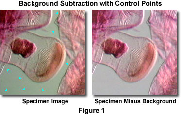
One or more of the control points may initially be superimposed over the specimen when the tutorial initializes. These points should be relocated to a background region to avoid introducing artifacts during creation of the background image. The control points should be distributed over the background to include as many of the intensity values as possible. A typical specimen with properly distributed control points is presented in Figure 1, along with the resulting image after background subtraction. The image illustrated in Figure 1 features an eosin-hematoxylin stained crab megalops developmental stage, which was captured in oblique illumination using the Olympus MIC-D digital microscope. When the microscope illuminator and condenser system is shifted away from the optical axis to introduce oblique lighting, background gradients are often observed in the resulting images. Application of a suitable background subtraction algorithm to correct these image defects should often be the first step in digital processing of captured images.

When a new specimen image is loaded into the interactive tutorial using the Choose A Specimen pull-down menu, the control point positions will always be reset to the periphery of the window containing the specimen image. The appearance of the background image is determined by the brightness levels of the pixels contained in a small neighborhood (9 to 81 pixels, depending upon the Control Point Size slider setting) bounded by the squares surrounding the control points. Visitors should explore repositioning the control points to create a new background image, and then examine the subtraction image that is produced by subtracting the background image from the specimen image. The best subtraction images result when control points are positioned so that the background image closely mimics that of the original specimen. As mentioned above, be careful to avoid placing control points on specimen regions to avoid artifacts in the resulting background subtraction image.

In transmitted light microscopy, the effects of nonuniformity in detector sensitivity and/or field illumination are often observed at very high magnification. Mottle, dirt, and a brightness gradient commonly appear in the image background, and these defects can seriously impair image contrast and mask important specimen detail. The removal of illumination defects and artifacts from images of highly magnified specimens is especially critical in video-enhanced contrast (VEC) microscopy. A method of background subtraction that is often employed in video microscopy involves capturing a background image by defocusing or by removing the specimen from the field of view. The captured background image is then repeatedly subtracted from each image that contains the specimen. This technique is not explored in the tutorial.

When it is not feasible to capture a background image in the microscope, a surrogate image can be created artificially by fitting a surface function to the background of the captured specimen image. This artificial background image can then be subtracted from the specimen image. By selecting a number of points in the image that are located in the background, a list of brightness values at various positions is obtained. The resulting information can then be utilized to obtain a least squares fit of a surface function that approximates the background. In the tutorial, eight adjustable control points are used to obtain a least squares fit of the background image with a surface function B(x, y) of the form:

where c(0) ... c(5) are the least squares solutions, and (x, y) represents the coordinates of a pixel in the fitted background image. The control points should be chosen so that they are evenly distributed across the image, and the brightness level at each control point should be representative of the background intensity. Placing many points within a small region of the image while very few or none are distributed into surrounding regions will result in a poorly constructed background image. In general, background subtraction is utilized as an initial step in improving image quality, although (in practice) additional image enhancement techniques must often be applied to the subtraction image in order to obtain a useful result.

The polynomial fitting methods explored in this tutorial can be combined with automatic histogram analysis of regions throughout the image to locate the brightest or darkest points for fitting. Alternative methods of background subtraction rely upon grayscale morphology (primarily erosion) operations to remove narrow (bright or dark) features and yield a background suitable for removal. Note that subtraction of the background from a digital image captured in the microscope is often not an appropriate processing step. Background subtraction is the method of choice for logarithmic detectors (such as analog video cameras and film), but not for linear detectors (many digital cameras and flatbed scanners), where the proper technique is to divide the image by the background.

---

BACK TO DIGITAL IMAGE CAPTURE AND PROCESSING

BACK TO THE OLYMPUS MIC-D DIGITAL MICROSCOPE

Questions or comments? Send us an email.

© 1995-2022 by Michael W. Davidson and The Florida State University. All Rights Reserved. No images, graphics, software, scripts, or applets may be reproduced or used in any manner without permission from the copyright holders. Use of this website means you agree to all of the Legal Terms and Conditions set forth by the owners.

This website is maintained by our
Graphics & Web Programming Team
in collaboration with Optical Microscopy at the
National High Magnetic Field Laboratory.

Last Modification Friday, Nov 13, 2015 at 01:19 PM

Access Count Since September 17, 2002: 16148

Visit the website of our partner in introductory microscopy education: