The perceived brightness of a digital image captured with an optical microscope is dependent not only upon the conditions of specimen illumination, but also on the sensitivity and linearity of the detector upon which the image was acquired. In addition, the characteristics of the display device (television, computer monitor, flat-screen display) where the digital image is viewed also affect the intensity distribution and interrelationship of contrast between light and dark regions in the specimen. The effects are characterized by a variable known as gamma, which is explored in this interactive tutorial.

	Interactive Java Tutorial
ATTENTION Our servers have detected that your web browser does not have the Java Virtual Machine installed or it is not functioning properly. Please install this software in order to view our interactive Java tutorials. You may download the necessary software by clicking on the "Get It Now" button below.

The tutorial initializes with a randomly selected specimen image, captured in the MIC-D digital microscope, appearing in the left-hand window entitled Specimen Image. Each specimen name includes, in parentheses, an abbreviation designating the contrast mechanism employed in obtaining the image. The following nomenclature is used: (BF), brightfield; (DF), darkfield; (OB), oblique illumination; and (RL), reflected light. Visitors will note that specimens captured using the various techniques available with the MIC-D microscope behave differently during image processing in the tutorial.

Appearing directly to the right of the Specimen Image window is a Transfer Function Graph that displays the relationship between the input and output pixel brightness values for the specimen. Beneath the transfer function graph window is a slider entitled Gamma Correction, which ranges in value from 0.45 to 2.5, and can be adjusted by translating the slider knob to the left (lower values) and right (higher values). To operate the tutorial, select a specimen from the Choose A Specimen pull-down menu and adjust the gamma correction control to observe how changing this parameter affects specimen appearance.

Modern CCD and CMOS imaging systems are often equipped with digital signal processing circuitry that can perform gamma correction through the use of look-up-tables. In a color video system, an identical correction function is applied to each of the red, green, and blue color channels, or to the Y channel in a YCbCr color video system. The integrated CMOS imaging sensor of the MIC-D digital microscope can perform both types of gamma correction through 128 preprogrammed correction curve settings. These corrections are user-configurable and can be adjusted to select one of several gamma correction curves. Gamma correction takes place in the analog signal-processing engine after image data has been collected from the photodiode array. The red, green, and blue components of the corrected signal are then mixed and fed into the analog-to-digital converter before being output to the video port.

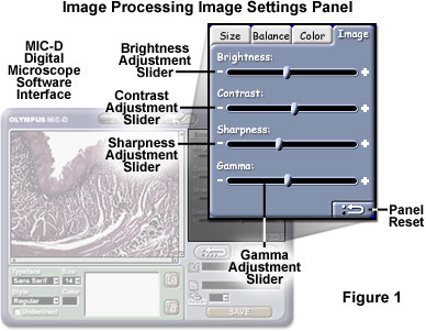
Gamma corrections can also be introduced at the software level in a majority of the popular digital image processing programs. The gamma correction feature of the MIC-D digital microscope software can be accessed from the Image Settings Panel tab of the image processing window, as illustrated in Figure 1. After all other image adjustments have been performed, including color balance, hue, saturation, sharpness, white and black balance, brightness and contrast, the image can be adjusted for optimal presentation on the computer monitor by utilizing the gamma correction slider.

The luminance generated by a display device is generally not a linear function of the applied voltage signal. This means that a typical cathode ray tube (CRT) will fail to correctly reproduce the brightness variations in a displayed digital image. Gamma correction is a process that can compensate for this effect.

In the ideal situation, the image generated by a CCD or CMOS image sensor is the result of a linear relationship between the intensity of light bathing the photodiode array and the signal gain and offset output to the display device. The relationship between the input illumination and the output signal is defined by the equation:

where S(o) is the gain of the output signal, K is a proportionality constant, E is the exposure time (related to intensity), and g is a measure of the device linearity (gamma). When the value of gamma is unity, the output signal is directly proportional to exposure time, or the intensity of light falling on the sensor. Thus, when gamma equals one, a double logarithmic plot of exposure time or intensity versus output current will yield a straight line (as illustrated by the Transfer Function Graph in the tutorial window when the Gamma Correction slider is in the center position). A majority of the video camera systems utilized in optical microscopy adhere to this relationship. In situations where gamma is less than 1, dark features in the image become brighter, but overall image contrast is reduced between the very bright and midtone grayscale values. When gamma has a value between 1 and 3, bright features become darker and overall contrast is increased, as illustrated in Figure 2. It should be noted that image contrast adjustments using gamma correction factors enable utilization of the entire range of pixels in the image. In comparison, histogram stretching and sliding techniques shift the brightness values, size, and position of the image pixel distribution.

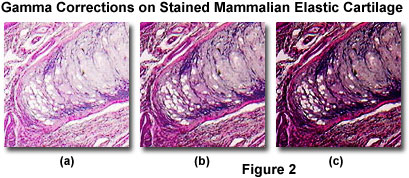
The images in Figure 2 demonstrate the effect of gamma corrections on typical specimens collected with the Olympus MIC-D digital microscope. This specimen is an eosin-hematoxylin stained thin section of mammalian elastic cartilage imaged and captured in brightfield illumination mode. When gamma is reduced to a value of 0.45 (Figure 2(a)), dark regions in the specimen are increased in brightness with a corresponding overall decrease in contrast between the light and dark areas. Increasing the gamma value to 2.5 (Figure 2(c)), suppresses dark features and accentuates the brightest highlights, leading to a sharp increase in contrast. For reference, the specimen is also illustrated (Figure 2(b)) with a gamma correction factor equal to 1 (linear).

Luminance is a measure of radiant light energy that is based upon the non-linear human visual response (logarithmic) to light. In many cases, very faint fluorescent images observed in the microscope are not accurately reproduced by film, a video camera, or CCD imaging device. This is because the human eye easily responds to specimens having low-amplitude, dim features in the same viewfield with bright highlights, but linear imaging devices are incapable of correctly reproducing the differences in luminance (and extremes in dynamic range) generated by these specimens. Exponential functions more closely match the logarithmic response of the human eye.

For cathode ray tube (CRT) display devices (computer monitors and televisions), the luminance produced at the face of the display is a power function, which is proportional to the voltage applied to the faceplate grid raised to an exponential power (usually about 2.5). The numerical value of the exponent of this power function is known as gamma, as discussed above for the behavior of digital imaging devices. Gamma correction involves adjusting the levels of the signal voltage to counteract the non-linear effects of monitor output. Figure 3 illustrates the non-linear output response curve (CRT Transfer Function) of a typical CRT along with a gamma correction curve that compensates for the non-linearity.

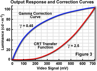
The mathematical form of gamma correction is a power function, whereby each input value is raised to a constant power. Ideally, the constant power of the correction function should be the reciprocal of the gamma of the CRT. This results in a correction curve that rises steeply from black (see the Gamma Correction Curve in Figure 3), which can elevate noise in the dark regions of the picture in a video system. In practice, a short linear segment is often introduced at the base of the transfer function in order to minimize dark noise. The growing popularity of flat-screen plasma and LCD monitors, which do not have gamma correction factors associated with electron guns, will help standardize calibration between the display and linear imaging devices.

When adjusting computer (and television) monitors that will be utilized for image processing, the transfer curve (gamma correction) depends, in part, on the brightness and contrast control settings on the monitor. In many cases, the control panel includes a potentiometer or on-screen setting for gamma that can affect the shape of the non-linear transfer curve. This enables the microscopist or digital artist to alter gamma correction to suit individual tastes and compensate for variability (and age) between monitors. Video displays can be calibrated with a grayscale test target containing bars or squares of varying gray levels. With the target visible on the screen, the various monitor controls are adjusted so the full range of brightness is visible without losing gray levels at either end. A properly calibrated image processing system will produce printed hard copies that appear identical to the on-screen image, which is an accurate representation of the digital image data.

---

BACK TO DIGITAL IMAGE CAPTURE AND PROCESSING

BACK TO THE OLYMPUS MIC-D DIGITAL MICROSCOPE

Questions or comments? Send us an email.

© 1995-2022 by Michael W. Davidson and The Florida State University. All Rights Reserved. No images, graphics, software, scripts, or applets may be reproduced or used in any manner without permission from the copyright holders. Use of this website means you agree to all of the Legal Terms and Conditions set forth by the owners.

This website is maintained by our
Graphics & Web Programming Team
in collaboration with Optical Microscopy at the
National High Magnetic Field Laboratory.

Last Modification Friday, Nov 13, 2015 at 02:19 PM

Access Count Since September 17, 2002: 17121

Visit the website of our partner in introductory microscopy education: