The term contrast refers to the amount of color or grayscale differentiation that exists between various image features in both analog and digital images. Images having a higher contrast level generally display a greater degree of color or grayscale variation than those of lower contrast. Image brightness (or luminous brightness) is a measure of intensity after the image has been acquired with a digital camera or digitized by an analog-to-digital converter.

This interactive tutorial explores the wide range of adjustment that is possible in digital image brightness and contrast manipulation, and how these variations affect the final appearance of the image. The tutorial initializes with a randomly selected specimen image, captured in the MIC-D digital microscope, appearing in the left-hand window entitled Specimen Image. Each specimen name includes, in parentheses, an abbreviation designating the contrast mechanism employed in obtaining the image. The following nomenclature is used: (BF), brightfield; (DF), darkfield; (OB), oblique illumination; and (RL), reflected light. Visitors will note that specimens captured using the various techniques available with the MIC-D microscope behave differently during image processing in the tutorial.

Adjacent to the Specimen Image window is a graph that displays the RGB/Grayscale Histogram of the microscope image (black or colored vertical bars), along with the intensity transfer function (black curve). Selecting the Red, Green, or Blue checkboxes will display the histogram for the corresponding color channel of the image in the RGB Histogram window (the default position is all three boxes checked). Two contrast adjustment mode controls are available in the tutorial, which correspond to specific contrast adjustment algorithms for Grayscale Contrast and RGB Contrast. Radio buttons are utilized to toggle between these contrast modes.

The contrast level of the specimen image is adjustable with the Contrast Level slider and/or a set of blue arrow buttons. To operate the tutorial, select an image from the Choose A Specimen pull-down menu, and vary the contrast level with the Contrast Level slider (or arrow buttons). Moving the slider to the left of the center position decreases image contrast, while moving the slider to the right increases image contrast. The slider can be translated either by dragging with the mouse cursor, or by clicking on the blue arrow buttons. The digital microscope image, histogram, and intensity transfer function graphs are continuously updated as the contrast level is varied with the slider. Visitors should note that the height of the histogram graph is scaled according to the number of pixels displayed at the top left of the vertical axis (labeled Pixel Count).

The specimen brightness level can be adjusted with the Brightness Level slider or its accompanying blue arrow buttons, in a manner analogous to that described above for the contrast controls. Moving the brightness slider to the left of center position decreases image brightness and shifts the histogram to lower input pixel brightness values. In contrast, translating the brightness slider to the right increases image brightness and shifts the histogram levels to higher input pixel brightness values.

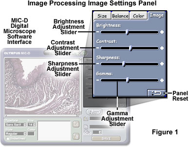
Brightness and contrast adjustments that are analogous to those described in the tutorial are available in the Olympus MIC-D digital microscope image processing software, as illustrated in Figure 1. After an image has been captured with the microscope's CMOS image sensor, it can be imported into the image processing software and adjusted with respect to brightness and contrast by varying the appropriate slider positions in the Image Settings Panel (see Figure 1). In a manner similar to that in the tutorial, moving the MIC-D software sliders to the left (towards the minus (-) icon) decreases brightness and contrast of the image displayed in the interface window, while moving the sliders to the right (closer to the plus (+) icon) increases values of these parameters. After the necessary brightness and contrast adjustments have been made to a digital image, the user can select another settings panel to apply the changes or click on the Panel Reset button to return the image to its original settings.

Brightness should not be confused with intensity (more accurately termed radiant intensity), which refers to the magnitude or quantity of light energy actually reflected from or transmitted through the specimen by the microscope illuminator. Instead, in terms of digital image processing, brightness is more properly described as the measured intensity of all the pixels comprising an ensemble that constitutes the digital image after it has been captured, digitized, and displayed. Pixel brightness is an important factor in digital images, because (other than color) it is the only variable that can be utilized by processing techniques to quantitatively adjust the image.

After a specimen has been sampled by the microscope optical system, each resolvable unit is represented either by a digital integer (provided the image is captured with a digital camera system) or by an analog intensity value on film (or a video tube). Regardless of the capture method, the image must be digitized to convert each continuous-tone intensity represented by the specimen into a digital brightness value. The accuracy of the digital value is directly proportional to the bit depth of the digitizing device. If two bits are utilized, the image can only be represented by four brightness values or levels. Likewise, if three or four bits are processed, the corresponding images have eight and 16 brightness levels, respectively. In all of these cases, level 0 represents black, while the upper level (3, 7, or 15) represents white, and each intermediate level is a different shade of gray.

These black, white, and gray levels are all combined in what constitutes the gray scale or brightness range of the image. A higher number of gray levels corresponds to greater bit depth and the ability to accurately represent a greater signal dynamic range. For instance, a 12-bit digitizer can display 4,096 gray levels, corresponding to a sensor dynamic range of 72 db (decibels). Color images are constructed of three individual channels (red, green, and blue) that have their own "gray" scales consisting of varying brightness levels for each color. The colors are combined within each pixel to represent the final image.

The contrast of a digital image is related to the RGB intensity (grayscale) values of the optical image and the accuracy of the digitizing device used to capture the optical image. The RGB intensity refers to the amount of red, green, and blue light energy actually reflected by, or transmitted through, the physical specimen at a given point. Although a number of factors play a role in specimen contrast, insufficient or non-uniform illumination and/or an incorrectly adjusted microscope can result in underexposure or blurring of specimen details, which is often a major cause of low contrast in digital images. The RGB intensity range utilized in construction of a color digital image is known as the intrascene dynamic range, and is a function of both the intensity range of the optical image and the accuracy of the camera used to capture the image. If the dynamic range of the digital image is severely limited by the camera's digitizer, then too few intensity levels will be available in each color channel to represent the subtle differences of intensity that may occur in the optical image. As a result, image contrast will suffer.

Deficiencies in digital image contrast can often be corrected by utilizing an intensity transformation operation, which is an algorithm designed to transform each input brightness value to a corresponding output brightness value via a transfer function. The purpose of the transfer function is simply to define a set of rules for assigning input pixel brightness values to output pixel brightness values. For images having low contrast, an intensity transformation can be employed to broaden the range of brightness values present in each color channel of the image, resulting in an overall increase in image contrast. However, in order for a contrast manipulation algorithm to perform properly, there must be sufficient variance in the pixel brightness values between pixel ensembles in the low-contrast image.

A chief advantage of the intensity transformation is that it affects only the color, but not the position, of a pixel. Also, unlike neighborhood operations, which determine an output pixel intensity color value as a function of the color values from a group of pixels in a neighborhood surrounding the input pixel, an intensity transformation determines the output pixel intensity color value as a function of the input pixel color value alone. For this reason, the algorithm is computationally very simple, and utilizing look-up tables (LUTs) for the intensity transfer function values further reduces processing time.

In the tutorial, the transfer function is a mathematical function whose graph is displayed as a black line or curve in the RGB Histogram window. When the Contrast Level slider is moved to the center position (default value), the intensity transfer function is simply an identity function (having a graph displayed as a straight line) that maps each input pixel intensity value to an identical output intensity value in each of the three color channels. The result is that each pixel's color or intensity value remains the same and no change in contrast occurs. As the slider is moved to the left of center position, the intensity transfer function compresses intensity values toward the center of the graph, resulting in a decrease of image contrast as differences between pixel brightness values are reduced or eliminated in each color channel of the image. When RGB Contrast is selected, this effect can also be seen in the red, green, and blue histograms of the image, which are compressed toward the center of the graph. Histogram compression corresponds to a reduction in the dynamic range of the resulting image in each color channel because fewer intensity levels are utilized per channel in the image display.

As the Contrast Level slider is moved to the right of the center position, the intensity transfer function increases the brightness variation among the mid-range intensity levels of each color channel of the image, while simultaneously decreasing the brightness variation among the low- and high-range intensity levels. The result is a general overall increase in image contrast, since the majority of brightness values in each color channel of an image will tend to occupy the mid-range of intensity levels of the histogram. This effect can be observed in red, green, and blue histograms of the processed image, which are gradually stretched to the boundaries. Histogram stretching corresponds to an increase in the dynamic range of each color channel of the image as more intensity levels become utilized in each channel of the displayed image. When the slider is moved to the extreme right of the center position, each histogram separates near the mid-range of the intensity levels, with all brightness values in each channel of the image being collected into the extremes (lowest and highest intensity values). The resulting effect is similar to posterization, where the number of colors in an image is reduced to the extent that the image takes on an artificial appearance.

---

BACK TO DIGITAL IMAGE CAPTURE AND PROCESSING

BACK TO THE OLYMPUS MIC-D DIGITAL MICROSCOPE

Questions or comments? Send us an email.

© 1995-2022 by Michael W. Davidson and The Florida State University. All Rights Reserved. No images, graphics, software, scripts, or applets may be reproduced or used in any manner without permission from the copyright holders. Use of this website means you agree to all of the Legal Terms and Conditions set forth by the owners.

This website is maintained by our
Graphics & Web Programming Team
in collaboration with Optical Microscopy at the
National High Magnetic Field Laboratory.

Last Modification Monday, Sep 18, 2017 at 01:08 PM

Access Count Since September 17, 2002: 20235

Visit the website of our partner in introductory microscopy education: