The word “noise” is used to describe portions of an image (or any electronic signal) that do not represent the original scene, but instead arise in the detector or electronics, or in some other way (e.g., flickering fluorescent lights, printing technology, etc.). There are at least three distinct categories of noise (see the Noise Types interactive tutorial) that are dealt with in different ways:

1. Random variations in pixel values, which appear as a speckle pattern superimposed on regions that should be uniform in brightness. These variations are produced by physical processes in the detector itself and in the associated electronics. Depending on camera design they may either affect each RGB channel independently, producing color variations, or may affect the pixel brightness without altering colors.

2. Shot noise, which appears as bright and/or dark pixels scattered across the image. Usually these are randomly placed but some may occur preferentially in rows or columns of pixels. Depending on camera design these may affect individual color channels producing colored pixels, or may affect all channels producing black or white pixels.

3. Interference, usually electronic but also possibly due to vibration or high frequency light sources (e.g., fluorescent lights) which can superimpose regularly spaced sets of lines across an image. This usually affects brightness rather than colors. Halftone printing of images also superimposes a pattern onto the image contents, and is dealt with using the same tools as interference.

In some examples below, the amount of speckle noise can be increased to relatively high levels to make it readily visible, but operating a camera at high gain (e.g., dim light) can produce this amount. Likewise the amount of shot noise can be made very high and most cameras would be rejected by the manufacturer if there were more than a few defective pixels of this type, but some kinds of microscopy can produce “dropouts” which are the same as shot noise, and dust on negatives also produces the same effects.

	Interactive Tutorial
Noise Types Learn about the various types of noise in images that often occur in images.

Other pages on this website discuss details of camera design and performance that are relevant to the sources of speckle and shot noise, explain why some sources are monochrome and some operate in individual color channels, why some speckle is additive and some multiplicative. The sources of these problems are not central to the issues here of image processing but some readers will find them interesting and relevant.

An often-used approach to reducing random speckle noise in images is a neighborhood smoothing operation. By averaging each pixel’s value with its neighbors, the random speckle in uniform regions tends to average out. However, this blurs edges and removes fine detail. Rather than simple averaging, a weighted averaging such as Gaussian smoothing produces the greatest amount of noise reduction for a given amount of blurring (or, conversely, the least blurring for a given amount of noise reduction). It is usually shown as a process applied directly to the pixels in the spatial domain, but is equivalent to an optimum low-pass filter applied in Fourier space (more about Fourier space filtering later on).

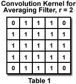
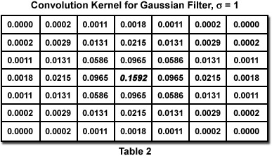
In the spatial domain, a convolution filter is applied by multiplying pixel values in a small neighborhood by numeric weights (called the kernel), adding up the sum and dividing by the sum of the weights, and using the result to replace the value of the central pixel. This procedure is applied to all pixels in the original image to produce a new image. Examples of averaging and Gaussian filters are shown in Tables 1 and 2. The latter has a profile that corresponds to a Gaussian or bell-shaped curve. Notice that Gaussian kernels quickly grow to be quite large, requiring many arithmetic operations.

As noted before, most filter operations should be applied to the monochrome brightness rather than to the individual R, G, B color channels. That is not always the case for noise reduction filters, depending on whether the noise is different in the various channels (which in turn depends on where it originates and on the camera design). The Speckle Noise Reduction By Spatial Averaging interactive tutorial compares various filtering kernels applied to noise in brightness or in the individual color channels.

	Interactive Tutorial
Speckle Noise Reduction By Spatial Averaging Evaluate the performance of neighborhood averaging in reducing speckle noise.

In addition to blurring edges and detail when applied to random speckle noise, convolution filters have even greater difficulties when applied to images with shot noise. In these instances, the extreme pixel values are averaged with their neighbors and while the magnitude of the noise is reduced, it is spread out into a larger area that may make it even more visually objectionable. The Shot Noise Reduction By Spatial Averaging interactive tutorial illustrates the effect of Gaussian filtering on shot noise.

	Interactive Tutorial
Shot Noise Reduction By Spatial Averaging Evaluate the performance of neighborhood averaging to reduce shot noise.

Because of these problems, convolution kernels are not a preferred method for dealing with shot noise or most cases of random speckle noise. Instead, a different neighborhood processing algorithm is used based on ranking the pixels in the neighborhood. This method is not a convolution and (unlike methods that use a kernel of weights) does not have a Fourier-space equivalent. Like convolutions, neighborhood ranking covers a variety of related techniques that are useful for many image processing operations, as will be shown below. For noise reduction, the particular procedure of interest is the median filter.

When the pixels in a neighborhood are ranked into order from brightest to darkest, the median value (in the middle of the ranked list) is placed in the central pixel location. This operation is applied to each pixel in the original image, to produce a new image in which the extreme pixel values are discarded. The Median Filtering of Monochrome Images interactive tutorial shows the application of a median filter with different neighborhood sizes to shot and speckle noise. Because no averaging is applied, the method does not blur edges. The median filter can, however, remove details that are smaller than the radius of the neighborhood. This offers a selective way to remove shot noise, dust and scratches, for instance.

	Interactive Tutorial
Median Filtering of Monochrome Images Explore the application of median filtering to shot and speckle noise in monochrome images.

The median filter works well and is straightforward to understand for monochrome images, but how should pixel values be ranked for a color image? One choice is to apply the median filter separately to each color channel, which works well for the case of shot noise that may be present in each channel separately. But if the median filter selects values in each channel that come from different pixels within the neighborhood, the resulting color shifts can produce problems, particularly near edges. The most common solution is to perform the ranking on the monochrome brightness value, and then copy the red, green and blue values from the selected neighborhood pixel. For multichannel and color images, there is also a vector median that plots each pixel’s values in color space, and defines as the median values the coordinates of the point whose distances to its neighbors is minimum. As shown in the Median Filtering of Color Images interactive tutorial, that method produces the best results for color images.

	Interactive Tutorial
Median Filtering of Color Images Explore the application of median filtering to shot and speckle noise in color images.

Although it does not shift edges, the median filter does remove fine lines and detail, and round corners. A more advanced version of this filter, which avoids these problems, is the hybrid median. This performs ranking in multiple sub-neighborhoods for each pixel, takes the median values from those rankings and performs a final ranking to select the final result. As shown in the Hybrid Median Filtering of Shot and Speckle Noise interactive tutorial, fine details are better preserved while the noise is removed.

	Interactive Tutorial
Hybrid Median Filtering of Shot and Speckle Noise Examine the application of hybrid median filtering to shot and speckle noise in color and monochrome images.

Periodic noise, arising from vibration, electronic interference, halftone printing, fluorescent lighting, or other causes is difficult or impossible to remove with neighborhood operations in the spatial or pixel domain, because it extends throughout the image. However, transforming the image to the Fourier or frequency domain often facilitates its removal. The Filtering Periodic Noise interactive tutorial illustrates the removal of electronic interference and halftone patterns. The Fourier transform power spectrum of the noisy image shows spikes (bright points indicating specific noise frequencies). Creating a mask to remove those spikes may be done either manually or using processing tools that will be introduced later on, applied to the image of the power spectrum itself. Once the spikes are removed, transforming the image back to the pixel domain recovers the image with the noise suppressed or removed.

	Interactive Tutorial
Filtering Periodic Noise Discover how Fourier transform filtering can be applied to the removal of interference and halftone patterns.

---

BACK TO INTRODUCTION TO DIGITAL IMAGE PROCESSING AND ANALYSIS

BACK TO MICROSCOPY PRIMER HOME

Questions or comments? Send us an email.

© 1998-2009 by Michael W. Davidson, John Russ, Olympus America Inc., and The Florida State University. All Rights Reserved. No images, graphics, scripts, or applets may be reproduced or used in any manner without permission from the copyright holders. Use of this website means you agree to all of the Legal Terms and Conditions set forth by the owners.

This website is maintained by our
Graphics & Web Programming Team
in collaboration with Optical Microscopy at the
National High Magnetic Field Laboratory.

Last modification: Tuesday, Sep 11, 2018 at 01:21 PM

Access Count Since July 20, 2006: 11335

For more information on microscope manufacturers,
use the buttons below to navigate to their websites: