A majority of the edge enhancement algorithms commonly employed in digital image processing often produce the unwanted side effect of increasing random noise in the image. Because it removes high-frequency spatial detail that can include random noise, the difference of gaussians algorithm is useful for enhancing edges in noisy digital images. This interactive tutorial explores application of the difference of gaussians algorithm to images captured in the microscope.

The tutorial initializes with a randomly selected specimen image (captured in the microscope) appearing in the left hand and center windows entitled Blurred Specimen (1) and Blurred Specimen (2), respectively. To operate the tutorial, select a specimen image from the Choose A Specimen pull-down menu. Each specimen name includes, in parentheses, an abbreviation designating the contrast mechanism employed in obtaining the image. The following nomenclature is used: (FL), fluorescence; (BF), brightfield; (DF), darkfield; (PC), phase contrast; (DIC), differential interference contrast (Nomarski); (HMC), Hoffman modulation contrast; and (POL), polarized light. Visitors will note that specimens captured using the various techniques available in optical microscopy behave differently during image processing in the tutorial.

The Blurred Specimen windows display the images that result from applying a Gaussian blur to the specimen image. The strength of the blur effect can be varied by using the s(1) and s(2) sliders, which will affect the appearance of the images in the left and center windows, respectively. Visitors should note that the value of the s(1) slider must be less than the value of the s(2) slider, and the tutorial will ensure this condition by automatically limiting the range of motion of the sliders. The Difference Image (1) - (2) window displays the image that results from subtracting the image appearing in the center window (Blurred Specimen (2)) from the image contained in the left-hand window (Blurred Specimen (1)). Visitors should explore how adjusting the slider combination affects the appearance of the blurred images and the difference image.

Difference of gaussians is a grayscale image enhancement algorithm that involves the subtraction of one blurred version of an original grayscale image from another, less blurred version of the original. The blurred images are obtained by convolving the original grayscale image with Gaussian kernels having differing standard deviations. Blurring an image using a Gaussian kernel suppresses only high-frequency spatial information. Subtracting one image from the other preserves spatial information that lies between the range of frequencies that are preserved in the two blurred images. Thus, the difference of gaussians is equivalent to a band-pass filter that discards all but a handful of spatial frequencies that are present in the original grayscale image. In its operation, the difference of gaussians algorithm is believed to mimic how neural processing in the retina of the eye extracts details from images destined for transmission to the brain.

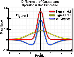
The plot of a cross section of two Gaussian curves with different standard deviations and their difference is illustrated in Figure 1. Note how the difference curve closely resembles that of the Laplacian, another commonly used edge enhancement algorithm.

As an image enhancement algorithm, the difference of gaussians can be utilized to increase the visibility of edges and other detail present in a digital image. A wide variety of alternative edge sharpening filters operate by enhancing high frequency detail, but because random noise also has a high spatial frequency, many of these sharpening filters tend to enhance noise, an undesirable artifact. The difference of gaussians algorithm removes high frequency detail that often includes random noise, rendering this approach one of the most suitable for processing images with a high degree of noise. A major drawback to application of the difference of gaussians algorithm is an inherent reduction in overall image contrast produced by the operation.

The sizes of the gaussian kernels employed to smooth the specimen image in the tutorial are indicated beneath the corresponding blurred images. When utilized for image enhancement, the difference of gaussians algorithm is typically applied when the size ratio of kernel (2) to kernel (1) is 4:1 or 5:1. The algorithm can also be used to obtain an approximation of the Laplacian of Gaussian when the ratio of s(2) to s(1) is roughly equal to 1.6. The Laplacian of Gaussian is useful for detecting edges that appear at various image scales or degrees of image focus. The exact values of s(1) and s(2) that are used to approximate the Laplacian of Gaussian will determine the scale of the difference image, which may appear blurry as a result.

---

BACK TO DIGITAL IMAGE PROCESSING TUTORIALS

Questions or comments? Send us an email.

© 1998-2022 by Michael W. Davidson and The Florida State University. All Rights Reserved. No images, graphics, scripts, or applets may be reproduced or used in any manner without permission from the copyright holders. Use of this website means you agree to all of the Legal Terms and Conditions set forth by the owners.

This website is maintained by our
Graphics & Web Programming Team
in collaboration with Optical Microscopy at the
National High Magnetic Field Laboratory.

Last modification: Tuesday, May 17, 2016 at 12:59 PM

Access Count Since February 19, 2002: 61644

Visit the websites of our partners in digital imaging education: