The Graphics Interchange Format (GIF), designed for encoding and storing digital images, is currently in worldwide use, being a popular medium for presentation of images by means of Web browser software. This interactive tutorial explores the compression of digital images using GIF algorithms, and how a lossy storage mechanism affects the final appearance of the image when interpolations are made from images having more than 256 colors.

The tutorial initializes with a randomly selected specimen image (captured in the microscope) appearing in the left-hand window entitled Specimen Image. Each specimen name includes, in parentheses, an abbreviation designating the contrast mechanism employed in obtaining the image. The following nomenclature is used: (FL), fluorescence; (BF), brightfield; (DF), darkfield; (PC), phase contrast; (DIC), differential interference contrast (Nomarski); (HMC), Hoffman modulation contrast; and (POL), polarized light. Visitors will note that specimens captured using the various techniques available in optical microscopy behave differently during image processing in the tutorial.

The number of distinct colors that appear in the unmodified specimen image is indicated beneath the Specimen Image window (this number varies with individual specimens). Appearing adjacent to this window is the Color-Reduced Image window, which displays the image that results from reducing the number of colors in the original specimen image. The number of distinct colors that appear in the color-reduced image is indicated beneath the Color-Reduced Image window. A slider (labeled Number of Colors) is available to vary the maximum number of colors that will be used in the color-reduced image, although the actual number of colors displayed in this image depends upon the techniques used in the color reduction and dithering. The Palette Selection Method pull-down menu can be employed to select from among the various color-reduction algorithms that are available in the tutorial. In a similar manner, the choice of dithering algorithm can be made using the Dithering Method pull-down menu. Visitors should observe the effects that the various palette selection and dithering algorithms have on the appearance of the specimen image.

The GIF format is useful for encoding and storing digital images of reduced file size, and relies on a lossy storage mechanism that operates by reducing the number of colors utilized to reconstruct the image. GIF images employ a color palette or look-up table (LUT), which consists of a list of colors that appear in the color-reduced image. The color of each pixel of the image is then represented by an index or offset into the palette table. Compression is achieved by applying the loss-less LZW (named after its creators, Lempel, Ziv, and Welch) compression algorithm to the image data, which is represented as a collection of palette indices. To limit the size of the stored GIF image file, the palette table is restricted to a maximum of 256 entries.

If the image to be compressed has more than 256 colors, then a color quantization or reduction algorithm must be applied to the image data prior to the compression operation. The process of color quantization involves selectively discarding colors from the image to reduce the amount of data. The selection process may be haphazard or it may be based upon considerations such as frequency of occurrence or perceptual significance of the colors in the image. The color selection process has a great deal of influence over the visual quality of the quantized image.

One of the simplest color reduction algorithms utilized prior to GIF compression is the uniform subdivision algorithm, which reduces the number of colors in an image by uniformly coarsening the intensity steps that are available in each of the red, green, and blue color channels.

This process is illustrated in Figure 1, where the intensity-range divisions that result from uniform subdivision are presented as a function of the total number of subdivisions. Note that as the number of subdivisions decreases, the gray-level intensity steps grow increasingly coarser. The uniform subdivision algorithm is an example of an indiscriminate approach to the color selection problem, because it ignores the issue of selecting colors that are the most important in reproducing the image. In the tutorial, the effects of applying the uniform subdivision algorithm to an image can be observed by selecting the Uniform Subdivision option from the Palette Selection Method pull-down menu. One interesting side effect of the uniform subdivision algorithm is an increase in the contrast of the color-reduced image. This effect becomes especially evident when the number of subdivisions per channel is low.

The popularity method of color reduction is one of several algorithms that have been created in an attempt to address the issue of color importance in image reconstruction. The design of this algorithm is intended to preserve those colors that occur most frequently in the image, but it is restricted in effectiveness by the fact that many images in microscopy have large areas of gray, black, or low-saturation colors. As a consequence, images that have been quantized by means of the popularity algorithm technique will often suffer from poor contrast, and important colors will often be absent from the quantized image, resulting in a loss of image detail. In the tutorial, the effects of applying the popularity algorithm to an image can be demonstrated by selecting the Popularity Method option from the Palette Selection Method pull-down menu.

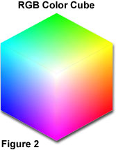
An algorithm that is more successful in identifying and preserving important colors in the color-reduced image is the median cut algorithm. The application of this technique is best explained in geometric terms using the RGB color cube concept, which is an additive color space model utilized by many modern video display devices to generate color video output. As illustrated in Figure 2, all of the colors occurring in the RGB color space can be represented by a three-dimensional matrix whose axes are the color components red, green, and blue. This matrix constitutes the RGB color cube.

A typical RGB image will utilize only a fraction of the total number of colors available in RGB color space. As presented in Figure 3, the colors that are used in an RGB image can be mapped onto an RGB color cube:

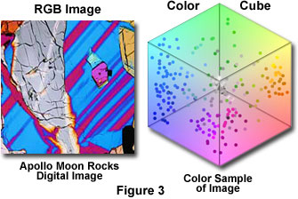
In the figure, the color cube on the right displays a map of the colors that occur in the polarized light image of a petrographic thin section located on the left-hand side of the figure. The lava section image contains a substantial number of blue, red, and gray tones, so an acceptable color palette for this image would concentrate more colors in these areas. The median cut algorithm attempts to accomplish this goal by successively dividing the color cube into regions of equal color count, where the color count is the sum of the histogram counts enclosed by each region of the color cube. The algorithm initializes by enclosing all of the colors in the image into a series of separate and smaller cubes defined within the boundaries of the larger color cube. Then, for each sub-cube, the minimum and maximum value of the red, green, and blue components is determined. The difference between these values is defined as the width of that color channel (or dimension), and the widest of these determines the dominant dimension among red, green, and blue. The sub-cube with the largest dominant dimension is then determined, and that sub-cube is split into two smaller cubes along the median point. This procedure divides the sub-cube into two halves so that equal numbers of colors are on each side, and the colors within the sub-cube are segregated into two groups depending on which half of the sub-cube they fall. The entire process is then repeated until the desired number of sub-cubes has been generated. The color for each sub-cube is then computed by averaging all of the colors that are contained in the sub-cube. The resulting set of colors constitutes the palette for the color-reduced image. Figure 4 illustrates the process.

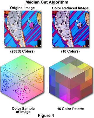
A majority of color images that have been quantized using the median cut algorithm demonstrate superior visual quality when compared to those quantized using uniform subdivision or the popularity method. The median cut algorithm requires a substantially greater processing time than the other two techniques (the amount of computational time required is dependent upon the number of colors processed). In the tutorial, the effects of applying the median cut algorithm to an image can be demonstrated by selecting the Median Cut option from the Palette Selection Method pull-down menu.

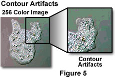
One problem that is often encountered with color quantization algorithms is quantization error, which stems from the fact that the color of a pixel in a quantized, or color-reduced, image is usually not identical to the color of the corresponding pixel in the original image. In addition, many regions of neighboring pixels having a range of colors in the original are reduced to the same color in the quantized image. This type of error is manifested in the form of unnatural color contours that appear in the quantized image (illustrated in Figure 5).

A simple means of correcting quantization error is to employ a technique known as error diffusion, a specific form of image dithering, which operates by distributing quantization error over a small neighborhood surrounding the target pixel. The algorithm functions by operating on each image pixel, in sequential order, starting from the top left pixel and proceeding from left to right to the bottom of the image. For each pixel, the error is computed between the red, green, and blue components that comprise both the original and quantized pixels. The error that is determined to occur at the central pixel is then distributed among the surrounding pixels. The amount of error that is distributed to the surrounding pixels is a function of the error diffusion algorithm that is employed. When designing algorithms for error transfer to a neighboring pixel, care must be exercised to ensure that the red, green, and blue components of the receiving pixel remain within the display range.

The Floyd-Steinberg error diffusion algorithm examines a small neighborhood of four pixels surrounding the central pixel, and distributes the error in the amounts indicated in Figure 6.

The large X in Figure 6 indicates the central pixel of the neighborhood. Two other error diffusion algorithms, the Jarvis-Judice-Ninke and the Stucki algorithm, use substantially larger neighborhoods that contain a greater number of pixels in order to spread the error distribution (as illustrated in Figure 7).

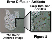
The performance of these three algorithms must be evaluated with respect to a particular application, but all are capable of success in reducing quantization error. Structure artifacts is a term for another common problem that is encountered with error diffusion image processing techniques. These artifacts tend to occur in regions of low intensity gradients such as background areas, and often break the visual continuity of features by introduction of artificial contour lines. Figure 8 illustrates typical structure artifacts that can arise when applying error diffusion algorithms.

In conclusion, the GIF format provides a substantial degree of image compression through the process of color reduction and loss-less LZW compression of the resulting image data. If an original image contains more than 256 distinct RGB colors, then quantization error and error diffusion artifacts can affect the accuracy of the information content when the image is compressed using one of the GIF algorithms. Consequently, when an image is to be stored for purposes of subsequent measurement or analysis, the GIF format is seldom used. This format is more useful for storing images intended for viewing on the Web, where short download times are an important (and often the primary) consideration. In addition, when capturing a large number of microscope images using a digital camera and a computer workstation, the GIF format can be used to create thumbnail images for rapid visual cataloging of specimens.

---

BACK TO DIGITAL IMAGE PROCESSING TUTORIALS

Questions or comments? Send us an email.

© 1998-2022 by Michael W. Davidson and The Florida State University. All Rights Reserved. No images, graphics, scripts, or applets may be reproduced or used in any manner without permission from the copyright holders. Use of this website means you agree to all of the Legal Terms and Conditions set forth by the owners.

This website is maintained by our
Graphics & Web Programming Team
in collaboration with Optical Microscopy at the
National High Magnetic Field Laboratory.

Last modification: Friday, Feb 12, 2016 at 11:06 AM

Access Count Since February 1, 2002: 65700

Visit the websites of our partners in digital imaging education: